We are using multiple imputation more frequently to “fill in” missing data in clinical datasets. Multiple datasets are created, models run, and results pooled so conclusions can be drawn.
We’ve put some improvements into Finalfit on GitHub to make it easier to use with the mice package. These will go to CRAN soon but not immediately.
See finalfit.org/missing.html for more on handling missing data.
Let’s get straight to it by imputing smoking status in a cancer dataset.
Install
devtools::install_github("ewenharrison/finalfit")
library(finalfit)
library(dplyr)
Create missing data for example
# Smoking missing completely at random

set.seed(1)

colon_s = colon_s %>%
  mutate(
    smoking_mcar = sample(c("Smoker", "Non-smoker", NA),
      dim(colon_s)[1], replace=TRUE,
      prob = c(0.2, 0.7, 0.1)) %>%
    factor() %>%
    ff_label("Smoking (MCAR)")
    )

# Smoking missing conditional on patient sex
colon_s$smoking_mar[colon_s$sex.factor == "Female"] =
  sample(c("Smoker", "Non-smoker", NA),
    sum(colon_s$sex.factor == "Female"),
    replace = TRUE,
    prob = c(0.1, 0.5, 0.4)
  )

colon_s$smoking_mar[colon_s$sex.factor == "Male"] =
  sample(c("Smoker", "Non-smoker", NA),
    sum(colon_s$sex.factor == "Male"),
    replace=TRUE, prob = c(0.15, 0.75, 0.1)
  )

colon_s = colon_s %>%
  mutate(
    smoking_mar = factor(smoking_mar) %>%
    ff_label("Smoking (MAR)")
  )
Check data
explanatory = c("age", "sex.factor",
  "nodes", "obstruct.factor",
  "smoking_mcar", "smoking_mar")
 dependent = "mort_5yr"
 colon_s %>%
  ff_glimpse(dependent, explanatory)

 Continuous
            label var_type   n missing_n missing_percent mean   sd  min quartile_25 median quartile_75  max
age   Age (years)    <dbl> 929         0             0.0 59.8 11.9 18.0        53.0   61.0        69.0 85.0
nodes       nodes    <dbl> 911        18             1.9  3.7  3.6  0.0         1.0    2.0         5.0 33.0

Categorical
                           label var_type   n missing_n missing_percent levels_n
sex.factor                   Sex    <fct> 929         0             0.0        2
obstruct.factor      Obstruction    <fct> 908        21             2.3        2
mort_5yr        Mortality 5 year    <fct> 915        14             1.5        2
smoking_mcar      Smoking (MCAR)    <fct> 828       101            10.9        2
smoking_mar        Smoking (MAR)    <fct> 719       210            22.6        2
                                             levels  levels_count   levels_percent
sex.factor                         "Female", "Male"      445, 484           48, 52
obstruct.factor            "No", "Yes", "(Missing)"  732, 176, 21 78.8, 18.9,  2.3
mort_5yr               "Alive", "Died", "(Missing)"  511, 404, 14 55.0, 43.5,  1.5
smoking_mcar    "Non-smoker", "Smoker", "(Missing)" 645, 183, 101       69, 20, 11
smoking_mar     "Non-smoker", "Smoker", "(Missing)" 591, 128, 210       64, 14, 23
Multivariate Imputation by Chained Equations (mice)
miceis a great package and contains lots of useful functions for diagnosing and working with missing data. The purpose here is to demonstrate how mice can be integrated into the Finalfit workflow with inclusion of model from imputed datasets in tables and plots.
Choose variables to impute and variables to impute from
finalfit::missing_predictorMatrix()makes it easy to specify which variables do what. For instance, we often do not want to impute our outcome or explanatory variable of interest (exposure), but do want to use them to impute other variables.
This is straightforward to code using the arguments drop_from_imputed and drop_from_imputer.
library(mice)

# Specify model
explanatory = c("age", "sex.factor", "nodes",
  "obstruct.factor", "smoking_mar")
dependent = "mort_5yr"

# Choose not to impute missing values
# for explanatory variable of interest and
# outcome variable.
# But include in algorithm for imputation.
predM = colon_s %>%
	select(dependent, explanatory) %>%
	missing_predictorMatrix(
		drop_from_imputed = c("obstruct.factor", "mort_5yr")
	)
Create imputed datasets
A set of multiple imputed datasets (mids) can be created as below. Various checks should be performed to ensure you understand the data that has been created. See here.
mids = colon_s %>%
  select(dependent, explanatory) %>%
  mice(m = 4, predictorMatrix = predM)    # Usually m = 10
Run models
Here we sill use a logistic regression model. The with.mids() function takes a model with a formula object, so use base R functions rather than Finalfit wrappers.
fits = mids %>%
  with(glm(formula(ff_formula(dependent, explanatory)),
    family="binomial"))
We now have multiple models run with each of the imputed datasets. We haven’t found good methods for combining common model metrics like AIC and c-statistic. I’d be interested to hear from anyone working on methods for this. Metrics can be extracted for each individual model to give an idea of goodness-of-fit and discrimination. We’re not suggesting you use these to compare imputed datasets, but could use them to compare models containing different variables created using the imputed datasets, e.g.
fits %>%
  getfit() %>%
  purrr::map(AIC)
[[1]]
[1] 1192.57

[[2]]
[1] 1191.09

[[3]]
[1] 1195.49

[[4]]
[1] 1193.729

# C-statistic
fits %>%
  getfit() %>%
  purrr::map(~ pROC::roc(.x$y, .x$fitted)$auc)
[[1]]
Area under the curve: 0.6839

[[2]]
Area under the curve: 0.6818

[[3]]
Area under the curve: 0.6789

[[4]]
Area under the curve: 0.6836
Pool results
Rubin’s rules are used to combine results of multiple models.
# Pool  results
fits_pool = fits %>%
  pool()
Plot results
Pooled results can be passed directly to Finalfit plotting functions.
# Can be passed to or_plot
colon_s %>%
  or_plot(dependent, explanatory, glmfit = fits_pool, table_text_size=4)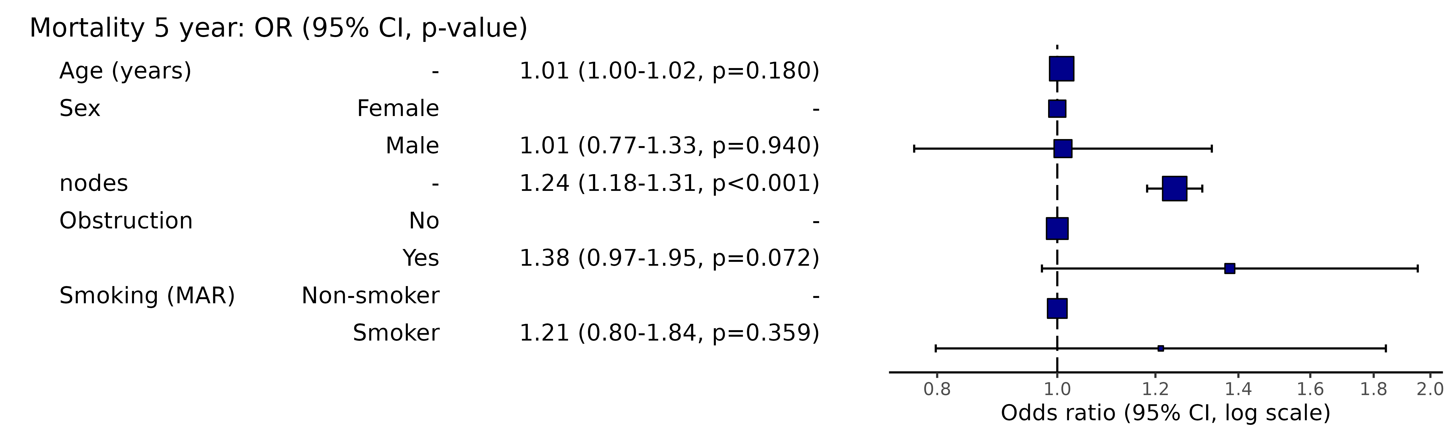
Put results in table
The pooled result can be passed directly to fit2df() as can many common models such as lm(), glm(), lmer(), glmer(), coxph(), crr(), etc.
# Summarise and put in table
fit_imputed = fits_pool %>%
  fit2df(estimate_name = "OR (multiple imputation)", exp = TRUE)
fit_imputed

         explanatory  OR (multiple imputation)
1                age 1.01 (1.00-1.02, p=0.212)
2     sex.factorMale 1.01 (0.77-1.34, p=0.917)
3              nodes 1.24 (1.18-1.31, p<0.001)
4 obstruct.factorYes 1.34 (0.94-1.91, p=0.105)
5  smoking_marSmoker 1.28 (0.88-1.85, p=0.192)
Combine results with summary data
Any model passed through fit2df() can be combined with a summary table generated with summary_factorlist() and any number of other models.
# Imputed data alone
## Include missing data in summary table
colon_s %>%
  summary_factorlist(dependent, explanatory, na_include = TRUE, fit_id = TRUE) %>%
  ff_merge(fit_imputed, last_merge = TRUE)

           label     levels       Alive        Died  OR (multiple imputation)
1    Age (years)  Mean (SD) 59.8 (11.4) 59.9 (12.5) 1.01 (1.00-1.02, p=0.212)
6            Sex     Female  243 (55.6)  194 (44.4)                         -
7                      Male  268 (56.1)  210 (43.9) 1.01 (0.77-1.34, p=0.917)
2          nodes  Mean (SD)   2.7 (2.4)   4.9 (4.4) 1.24 (1.18-1.31, p<0.001)
4    Obstruction         No  408 (56.7)  312 (43.3)                         -
5                       Yes   89 (51.1)   85 (48.9) 1.34 (0.94-1.91, p=0.105)
3                   Missing   14 (66.7)    7 (33.3)                         -
9  Smoking (MAR) Non-smoker  328 (56.4)  254 (43.6)                         -
10                   Smoker   68 (53.5)   59 (46.5) 1.28 (0.88-1.85, p=0.192)
8                   Missing  115 (55.8)   91 (44.2)                         -
Combine results with other models
Models can be run separately, or using the finalfit()wrapper including the argument keep_fit_it = TRUE.
colon_s %>%
finalfit(dependent, explanatory, keep_fit_id = TRUE) %>%
ff_merge(fit_imputed, last_merge = TRUE)
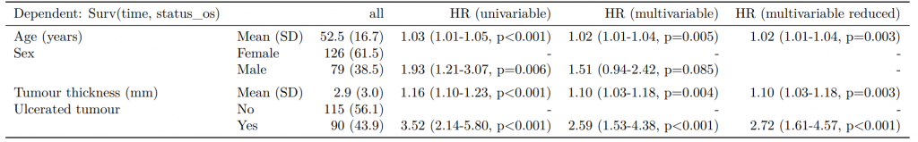
Dependent: Mortality 5 year Alive Died OR (univariable) OR (multivariable) OR (multiple imputation)
1 Age (years) Mean (SD) 59.8 (11.4) 59.9 (12.5) 1.00 (0.99-1.01, p=0.986) 1.02 (1.00-1.03, p=0.010) 1.01 (1.00-1.02, p=0.212)
5 Sex Female 243 (47.6) 194 (48.0) - - -
6 Male 268 (52.4) 210 (52.0) 0.98 (0.76-1.27, p=0.889) 0.88 (0.64-1.23, p=0.461) 1.01 (0.77-1.34, p=0.917)
2 nodes Mean (SD) 2.7 (2.4) 4.9 (4.4) 1.24 (1.18-1.30, p<0.001) 1.25 (1.18-1.33, p<0.001) 1.24 (1.18-1.31, p<0.001)
3 Obstruction No 408 (82.1) 312 (78.6) - - -
4 Yes 89 (17.9) 85 (21.4) 1.25 (0.90-1.74, p=0.189) 1.26 (0.85-1.88, p=0.252) 1.34 (0.94-1.91, p=0.105)
7 Smoking (MAR) Non-smoker 328 (82.8) 254 (81.2) - - -
8 Smoker 68 (17.2) 59 (18.8) 1.12 (0.76-1.65, p=0.563) 1.25 (0.82-1.89, p=0.300) 1.28 (0.88-1.85, p=0.192)Model missing explicitly in complete case models
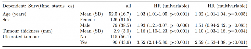
A straightforward method of modelling missing cases is to make them explicit using the forcats function fct_explicit_na().
library(forcats)
colon_s %>%
mutate(
smoking_mar = fct_explicit_na(smoking_mar)
) %>%
finalfit(dependent, explanatory, keep_fit_id = TRUE) %>%
ff_merge(fit_imputed, last_merge = TRUE)
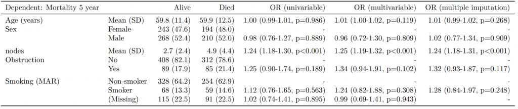
Dependent: Mortality 5 year Alive Died OR (univariable) OR (multivariable) OR (multiple imputation)
1 Age (years) Mean (SD) 59.8 (11.4) 59.9 (12.5) 1.00 (0.99-1.01, p=0.986) 1.01 (1.00-1.02, p=0.119) 1.01 (1.00-1.02, p=0.212)
5 Sex Female 243 (47.6) 194 (48.0) - - -
6 Male 268 (52.4) 210 (52.0) 0.98 (0.76-1.27, p=0.889) 0.96 (0.72-1.30, p=0.809) 1.01 (0.77-1.34, p=0.917)
2 nodes Mean (SD) 2.7 (2.4) 4.9 (4.4) 1.24 (1.18-1.30, p<0.001) 1.25 (1.19-1.32, p<0.001) 1.24 (1.18-1.31, p<0.001)
3 Obstruction No 408 (82.1) 312 (78.6) - - -
4 Yes 89 (17.9) 85 (21.4) 1.25 (0.90-1.74, p=0.189) 1.34 (0.94-1.91, p=0.102) 1.34 (0.94-1.91, p=0.105)
8 Smoking (MAR) Non-smoker 328 (64.2) 254 (62.9) - - -
9 Smoker 68 (13.3) 59 (14.6) 1.12 (0.76-1.65, p=0.563) 1.24 (0.82-1.88, p=0.308) 1.28 (0.88-1.85, p=0.192)
7 (Missing) 115 (22.5) 91 (22.5) 1.02 (0.74-1.41, p=0.895) 0.99 (0.69-1.41, p=0.943) -Export tables to PDF and Word
As described elsewhere, knitr::kable() can be used to export good looking tables.